15 Convolutional Neural Network
CNN are sparsely connected multilayer network with parameter sharing. One motivation for the introduction of CNN is that for image data a standard fully connected architecture would require vast numbers of parameters due to the high-dimensional nature of images. To mitigate this, we want to create an inductive bias based on four concepts:
- Hierarchy: neural network learn hierarchical representations of the input
- Locality: feature can be detected in a local region of an image
- Equivariance: the neural network must be able to generalize what it has learned in one location to all possible locations in the image
- Invariance: the predictions should be unchanged under one or more transformations of the input variables
15.1 Structure
15.1.1 Convolutional Layer
The neuron in a layer takes as input the pixel values from a small rectangular region called receptive field of that unit, and it captures the notion of locality. Weight values associated with this unit will learn to detect some useful feature.
The weights form a two-dimensional grid called filter or kernel. During the forward pass, the unit will act as a feature detector that signals when it find a sufficiently good match to its kernel.
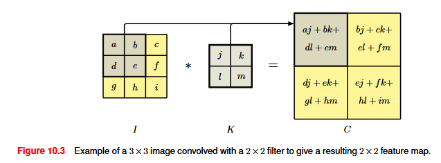
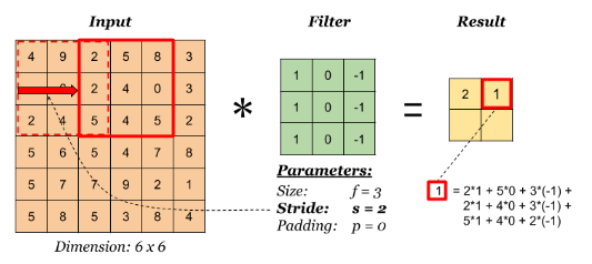
To encode the equivariance, we can replicate the same hidden-unit weight values at multiple locations across the image, to form a feature map, in which all the units share the same weights. This transformation is an example of a convolution: given an image I with pixel intensities I(j, k), j, k indices, and a filter K with pixel values K(l, m), l, m indices, the feature map C has activation values given by C(j, k) = \sum_l \sum_m I(j+l, k+m) K(l,m)
This is strictly speaking called a cross-correlation.
Now, some hyperparameters:
- Padding: If the image has dimensionality J \times K pixels and we convolve with a kernel of dimensionality M \times M the resulting feature map has dimensionality (J - M + 1) \times (K - M + 1). In some cases we want the feature map to have the same dimensions as the original image. This can be achieved by padding the original image with additional pixels around the outside. If there is no padding, so that P = 0, this is called a valid convolution. When the value of P is chosen such that the output array has the same size as the input, corresponding to P = \dfrac{M - 1}{2}, this is called a same convolution, because the image and the feature map have the same dimensions.
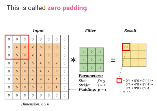
- Stride: Sometimes we wish to use feature maps that are significantly smaller than the original image. One way to achieve this is to use strided convolutions in which, instead of stepping the filter over the image one pixel at a time, it is moved in larger steps of size S, called the stride.
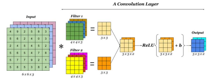
We can easily extend convolutions to cover multiple channels by extending the dimensionality of the filter. Simply, we introduce a filter described by a tensor of dimensionality M \times M \times C, comprising a separate M \times M filter for each of the C channels.
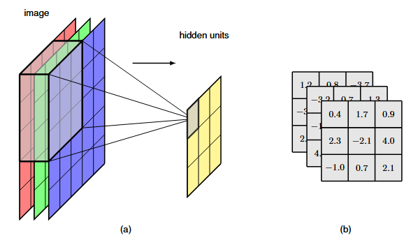
In every convolutional layer, we can include multiple filter, in which each filter has its own independent set of parameters giving rise to its own independent feature map.
15.1.2 Pooling
A convolutional layer encodes translation equivariance: if a small patch of pixels is moved to a different location in the image, the associated outputs of the feature map will move to the corresponding location in the feature map. This is obviously desirable, but small changes relative to the original location should not affect the classification, so we want invariance to such small changes. This is achieved using pooling to the output of a convolutional layer. The output of a pooling unit is a simple, fixed function of this inputs, and so there are no learnable parameters. Again, there is a choice of filter size and of stride length.
Some pooling functions are:
- max-pooling, in which each unit simply output the max function applied to the input values.
- average pooling, in which the pooling function computes the average of the values from the corresponding receptive field in the feature map
Pooling can also be used to reduce the dimensionality of the representation by down-sampling the feature map. It is usually applied to each channel of a feature map independently.
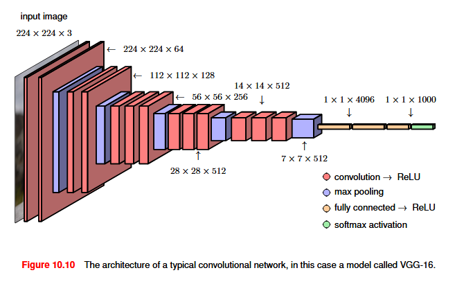
15.1.3 Fully connected layers
In many applications, the output units of the network need to make predictions about the image as a whole, and so they need to combine information from across the whole of the input image. This is typically achieved by introducing one or two standard fully connected layers as the final stages of the network.
A complete CNN therefore comprises multiple layers of convolutions interspersed with pooling operations, and often with fully connected layers in the final stages of the network. There are many choices to be made in designing such an architecture including the number of layers, the number of channels in each layer, the filter sizes, the stride widths, and multiple other such hyperparameters.